Data Science for Agriculture
How to manage and manipulate data for agricultural research

Now that you have all the data in R, it’s time to prepare the data for creating your map. In order to create your map you need to have all of your layers clipped to the same extent and using the same projection.
Use the extent function to check the geographic extent of the data layers
for Oklahoma county boundaries, NOAA climate divisions, Oklahoma elevation, and
Oklahoma Mesonet station locations.
You note that all the layers seem pretty close except for the NOAA climate
divisions and you realize that you forgot to subset that layer to include only
climate divisions for Oklahoma. Use the subset function to exclude any
polygons that are not in Oklahoma and assign the resulting
SpatialPolygonsDataFrame to a new R object. Check the extent of the new data
layer.
Now that the extents are good, you need to check the projections. Use crs
to check the projections of your data layers for Oklahoma county boundaries,
Oklahoma climate divisions, Oklahoma elevation, and Oklahoma Mesonet station
locations.
You notice that the output from crs is different for your layers. To make
sure that everything lines up properly you decide to transform each layer to
match the CRS as specified for the Oklahoma county boundaries layer. Use spTransform to transform all your vector data layers to the CRS from the Oklahoma boundaries layer. Use crs to assign the proper CRS specification to your raster layer. Check all CRS specifications using crs.
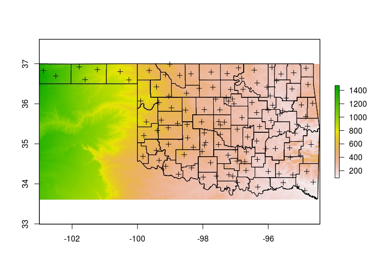
Plot all data layers starting with Oklahoma elevation. (Hint:
use add=TRUE to overlay each data layer)
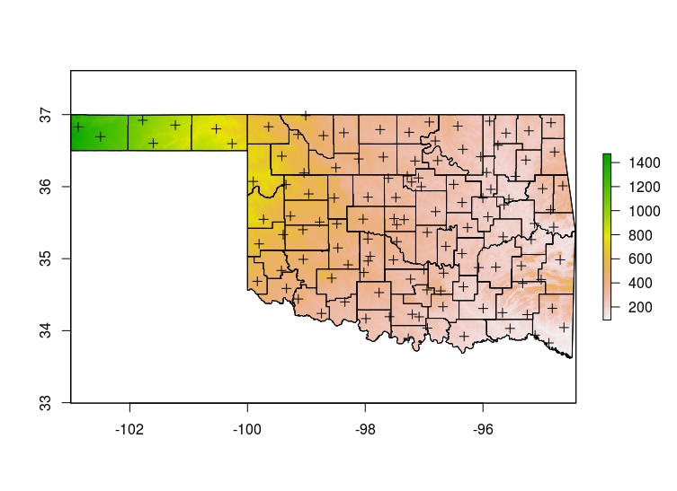
In looking at your preliminary map, you realize that you need to remove the
areas of the Oklahoma elevation data layer that are beyond the state boundary.
Use the mask function to create a new data layer that contains only values
that are within the state boundary. Plot all data layers starting with your
new elevation data layer.
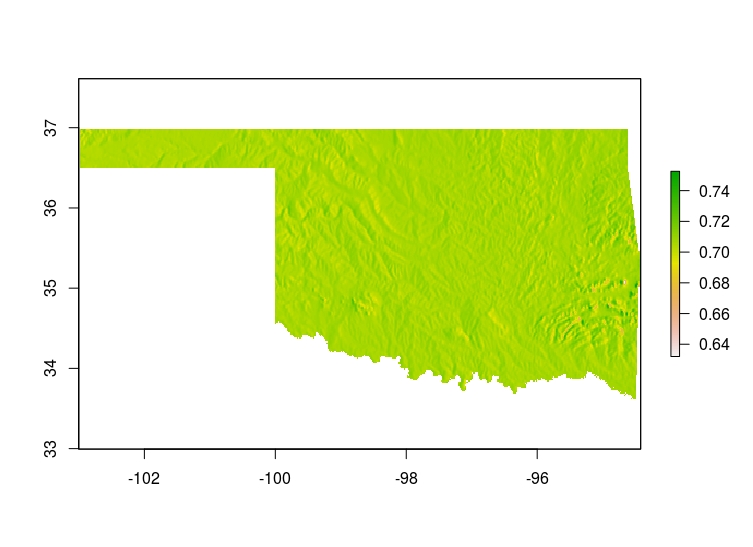
You’re feeling pretty proud of your map so you show it off to your
office-mate. He suggests that a hillshade plot for your elevation data might
highlight the topography better. After some searching, you find that you can
create a hillshade plot using the hillShade function. To do that, you’ll
need to use the terrain function to calculate the slope and aspect and assign
them to objects that you can provide as arguments to hillShade. Create a
hillshade data layer using the slope and aspect calculated from the elevation
data and plot the result. (Hint: use 45 for the angle and 270 for the
direction arguments to hillShade)