Data Science for Agriculture
How to manage and manipulate data for agricultural research

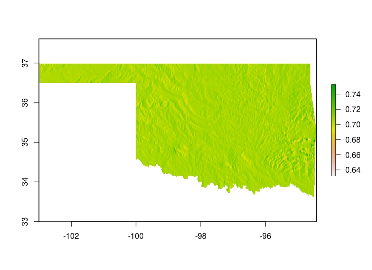
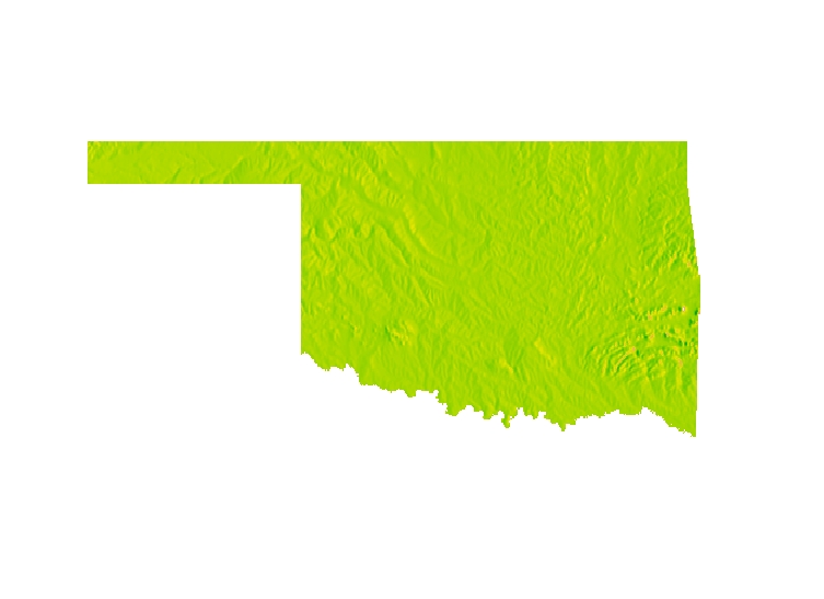
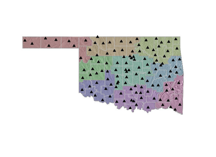
Your data layers are ready to be combined into your final map.
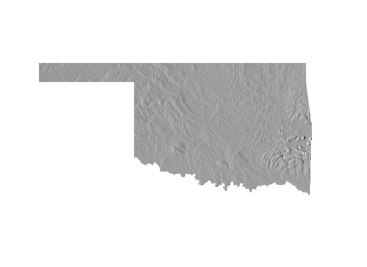
Plot the hillshade data layer.
The legend of the hillshade plot is not very informative and somewhat
distracting so you decide it can be removed. You also decide that the axes and
bounding box are unncessary. Plot the hillshade layer again removing the axes,
bounding box, and legend. (Hint: use box=FALSE to get rid of the bounding
box)
Because you intend to overlay other layers on top of the hillshade layer, you
decide it would be better to have the hillshade in grayscale instead of color.
Use the gray function and the col argument to plot to plot the hillshade
layer in grayscale. (Hint: using 0:100/100 for the level argument to
gray should give you a nice contrast).
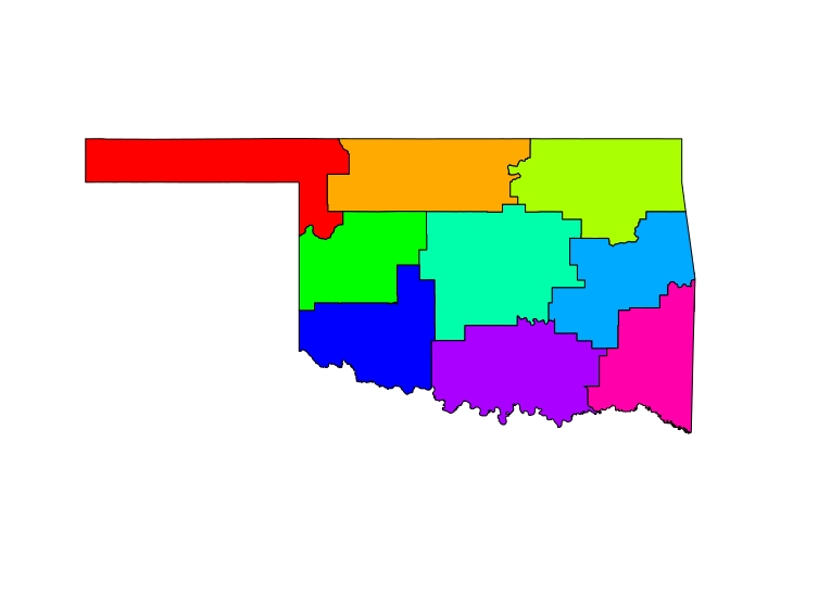
Add the Oklahoma climate divisions to the map using the rainbow function
and the col argument to plot. Be sure to specify the proper number of
colors to correspond to the number of climate divisions when you call rainbow.
You realize that in order to see the elevation you will need to increase the
transparency of the colors for the climate divisions layer. Use the alpha
argument to the rainbow function to make the colors more transparent and
replot the elevation and climate division layers. (Hint: an alpha value of
about 0.15 should be about right.)
Now you are ready to add the Oklahoma county boundaries layer. Use plot to
add this layer to the plot. The county boundaries are really more background
context for the map, so use the border argument to set the color for the
boundary lines to “gray”.
You are now ready to add your Oklahoma Mesonet station locations to your map.
Add the Oklahoma Mesonet station layer to your map. Use the pch argument to
set the point character to a filled triangle.