Producing Documents with R

Learning Objectives

Following this assignment students should be able to:

Create an R Markdown document

Read data into R directly from an Excel spreadsheet

Embed R code for data analysis within a document

Embed R code to generate and display figures and tables within a document

Create a BibTex/BibLaTeX bibliography database

Generate citations and references within an R Markdown document

Reading

Topics
- R Markdown
Readings

Exercises

-- R Markdown Basics --

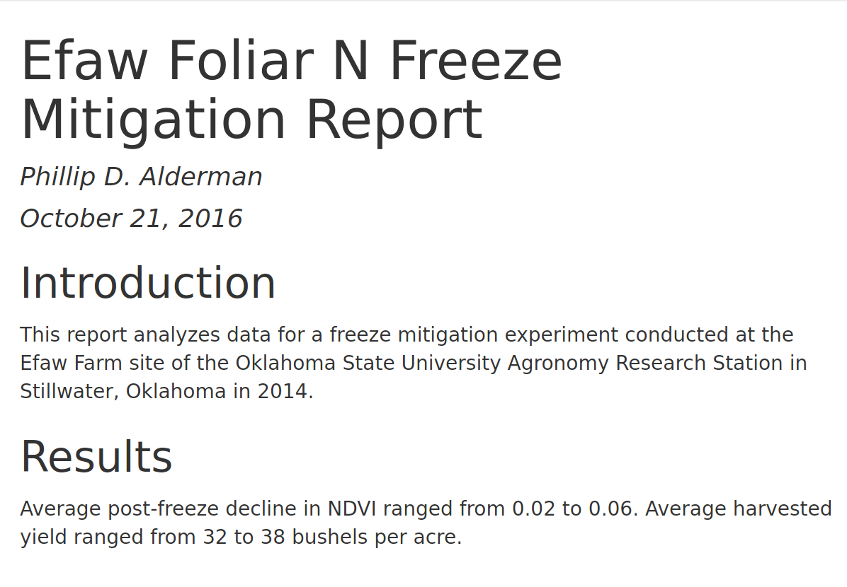
Dr. Raun has asked you to do some preliminary analysis of some data from a study conducted to investigate the interactions between foliar N application and frost. You decide to put some of your new R skills to use and produce the report using R Markdown.

To do so, open a new R Markdown file within R Studio. Use “Efaw Foliar N Freeze Mitigation Report” for the title and your name for the author. The new file will contain an example template for an R Markdown document. Click on the Knit HTML button to compile your R Markdown document. Compare the resulting output with the R Markdown script. Read through the template R Markdown file and the resulting output for an explanation of how R Markdown works.

Next, create a subdirectory named data and download the data you will use (Efaw_Freeze2014.xlsx). Because the data are in an MS Excel spreadsheet, you will want to use the handy read.xlsx() function to read in the data. To do so, you will need to install the xlsx R package first.
1. Within your R Markdown file, create a new R code block with the chunk name “read_data” that loads the xlsx package using library() and reads in the data using the read.xlsx() function. (Hint: You will need to use sheetIndex=1. Also, don’t modify the Excel file to read it in. Use the startRow and endRow options within read.xlsx() to read in the header row and data.)
2. Add a line to the code block that changes the variable for the change in NDVI to all positive values.
3. Add a line to the code block that uses the as.factor() function to convert the treatment column from a numeric column to a factor column.
4. Add a line that summarizes your data frame using the summary() function.
5. The displayed R code and summary output are useful as you were checking that the data were read in properly, but you probably don’t want them in your final report. Use the echo=FALSE and include=FALSE options to the code chunk to keep these from being displayed in your document.
6. Below your “read_data” code chunk, add a header entitled Introduction to your document using the ## notation and add a sentence below introducing the overall purpose of the report.
[click here for output]
-- R Markdown Data Analysis --

This is a follow-up to R Markdown Basics.

You now have all the data read into R and you are ready to begin your analysis. You consult with a colleague who has done this kind of work for Dr. Raun before and are delighted to discover that she uses R, too. She shares a function with you that she wrote to automate parts of the analysis:
```
analyze <- function(formula,data){
  library(agricolae,quietly=TRUE)
  fit.lm <- lm(formula,data=data)
  fit.anova <- anova(fit.lm)
  fit.test <- LSD.test(y=data[,as.character(formula[[2]])],
                         trt=data[,as.character(formula[[3]])],
                         DFerror=tail(fit.anova$Df,1),
                         MSerror=tail(fit.anova$`Mean Sq`,1))
  return(fit.test$groups)
}
```
You notice that the function loads the agricolae package, which you have not used before. You make a note that you’ll need to install it before you can use the function.
1. Add a section to your R Markdown file entitled Results and copy the function code into a new R code chunk with the name “define_analysis_function”. Knit your document and inspect the output. Set the code chunk options so that neither R code nor any output are displayed for this code chunk.
2. Create a new code chunk named “run_analysis” and add R code to use the analyze() function to calculate treatment means and mean groupings using Fisher’s LSD for post-freeze decline in NDVI and harvested yield. Assign each of these to a separate object. Set the code chunk options so that neither R code nor any output are displayed for this code chunk.
3. Use in-line R code chunks to write a sentence for each variable that states the minimum and maximum mean values for NDVI decline, rounded to the 2^nd^ decimal place, and for harvested yield, rounded to the nearest bushel.
[click here for output]
-- R Markdown Figures --

This is a follow-up to R Markdown Data Analysis.

Now that you have completed your analysis, you want to visualize the analysis for more user-friendly presentation. You decide to use the ggplot() to create some bar graphs that will display the data.
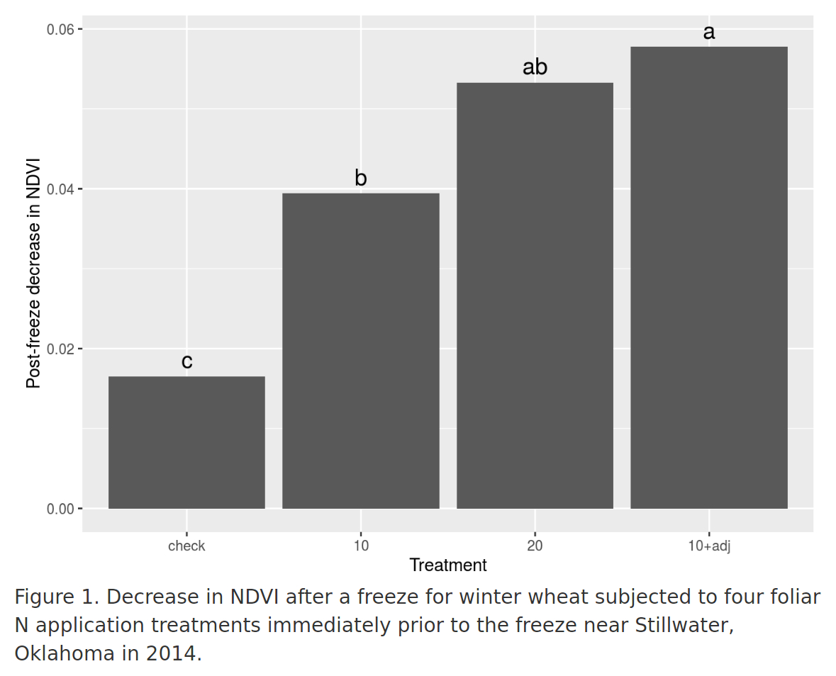
1. Add an R code chunk named “NDVI_plot” with the code needed to produce a barplot of the treatment means for the post-freeze NDVI decline. Be sure to label the axes appropriately.
2. Use geom_text() to add labels to the bars to indicate significant differences between treatment means. Use the vjust, nudge_y, and size arguments for geom_text() to size and position the labels appropriately.
3. Add a sensible caption to the figure (including a figure number) using the fig.cap chunk option.
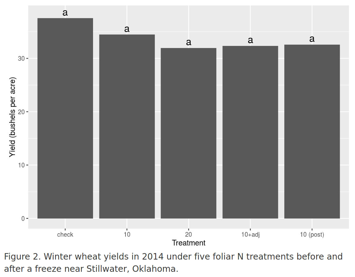
4. Add a new R code chunk named “yield_plot” with R code to produce an equivalent figure for the yield data. Be sure to include appropriate axis labels, bar labels for statistically significant differences, and a suitable figure caption.
5. Set the echo chunk option for both code chunks so that no R code is displayed in the final output.
6. Add a sentence or two to your Results section describing the figures and referencing them appropriately.
[click here for output] [click here for output]
-- R Markdown Tables --

This is a follow-up to R Markdown Figures.

Because you are unsure how Dr. Raun will prefer the data to be presented, you decide to include the data in a table, as well.
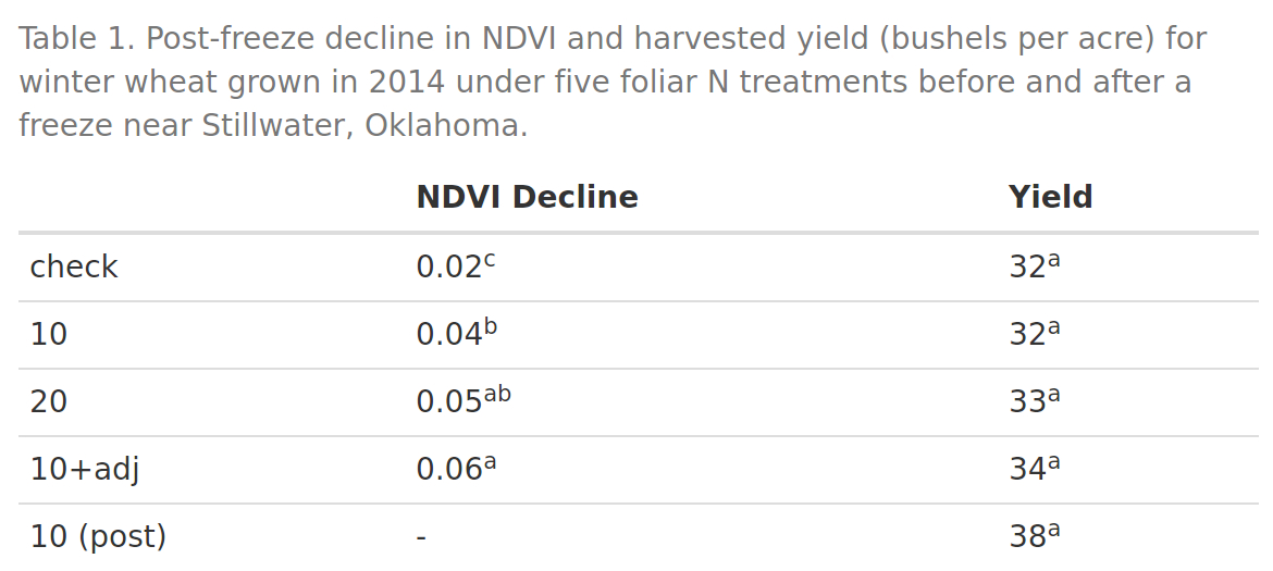
1. Within a new code chunk named “results_table”, create a data frame that has columns with treatment means for post-freeze NDVI decline and yield. Set the column names to “NDVI Decline” and “Yield”. Set the row names to abbreviations for the corresponding treatments (i.e. not just treatment number). (Hint: I suggest you round the values appropriately and then convert these to text using paste(). You also will need to add a dash in your NDVI column for the missing treatment level)
2. Add the statistical significance labels to your results table using the paste0() function.
3. Modify your code to add Markdown notation to make the significance labels superscript.
4. Use the kable() function to generate your table.
5. Use the caption argument to the kable() function to add a suitable caption for the results table.
6. Set the code chunk options so that your R code is not displayed.
[click here for output]
-- R Markdown References --

This is a follow-up to R Markdown Tables.

Your next steps as you write up your report are to document your methods with proper citations and to discuss your results while citing appropriate references. Fortunately, R Markdown provides a useful framework for handling citations. Create a new text file with R Studio using the name “bibliography.bib” (“.bib” is the file extension for a BibTeX or BibLaTeX bibliography database). This is where you will put the bibliographic information for each citation.
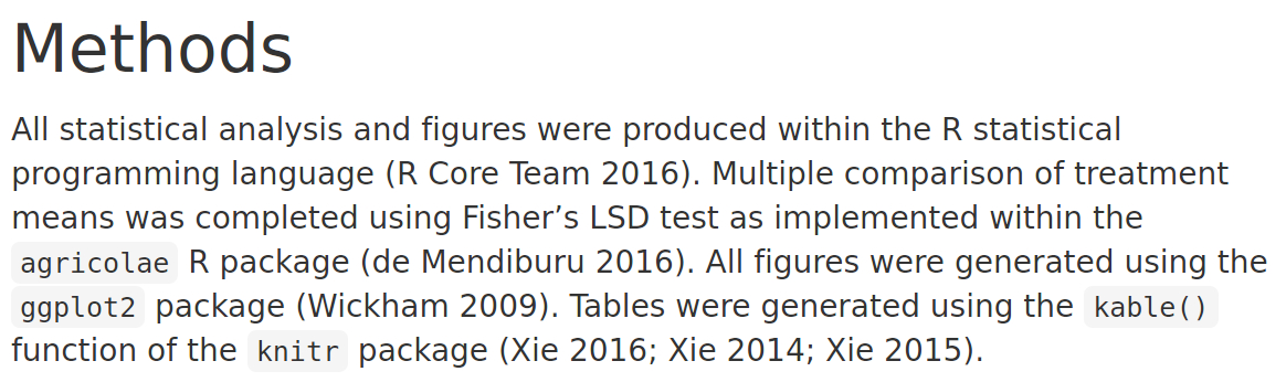
1. Add a Methods section to your document and describe the basic methods used for your analysis. Be sure to mention that you used the R statistical programming language and mention the names of the R packages you used to analyze the data and produce the figures.
2. In your console, type the command citation(). The resulting output will include a BibTeX entry for R that begins with @Manual and is enclosed by curly brackets {}. Copy the BibTeX entry into your “bibliography.bib” file and add a suitable citation key (such as Rproject) between the first { and the ,. Using the same citation key, add a citation to your R Markdown file in the Methods section immediately after where you mention using R.
3. Return to the console and use the citation() function to generate BibTeX entries for each of the packages used in your analysis. Add a unique citation key to each entry and use the key in your Methods section to cite each package appropriately.
4. Within your R Markdown file, scroll to the end of the Results section and start a new section entitled Discussion. You recall that Dr. Raun mentioned a paper he published on late-season foliar N application for wheat in 2002 so you decide to compare those results to your current results. Go to Google Scholar and search for the paper using the query author:Raun late-season foliar nitrogen wheat. You are confident you will cite this paper, so click the Cite link under the appropriate entry in the search results. Then click the BibTeX link at the bottom of the pop-out window. Copy the resulting BibTeX entry into your “bibliography.bib” file. Feel free to change or shorten the citation key, if you like.
5. Briefly read over the paper and write one or two sentences in the Discussion section comparing your results to those of the paper. Be sure to include a citation for the paper.
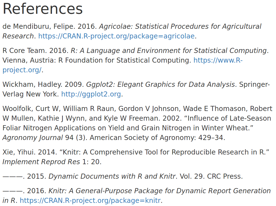
6. Once you knit your document, you notice that you’ve forgotten to add a header for the References section. Add this as the last line of your R Markdown file.
[click here for output] [click here for output] [click here for output]

Data Science for Agriculture

Assignment

Learning Objectives

Reading

Exercises

-- R Markdown Basics --

-- R Markdown Data Analysis --

-- R Markdown Figures --

-- R Markdown Tables --

-- R Markdown References --