Learning Objectives

Following this assignment students should be able to:

• Import existing spatial datasets into R
• Read-in and convert raw data to a spatial data layer
• Manipulate spatial data based on data attributes
• Transform spatial data layers for subsequent analysis
• Combine spatial data layers to produce a map

Reading

• Topics

  • R spatial

• Readings

• Introduction to Working With Vector Data in R
• Introduction to Working With Raster Data in R
• Spatial Cheatsheet

Exercises

1. -- Importing Spatial Data --

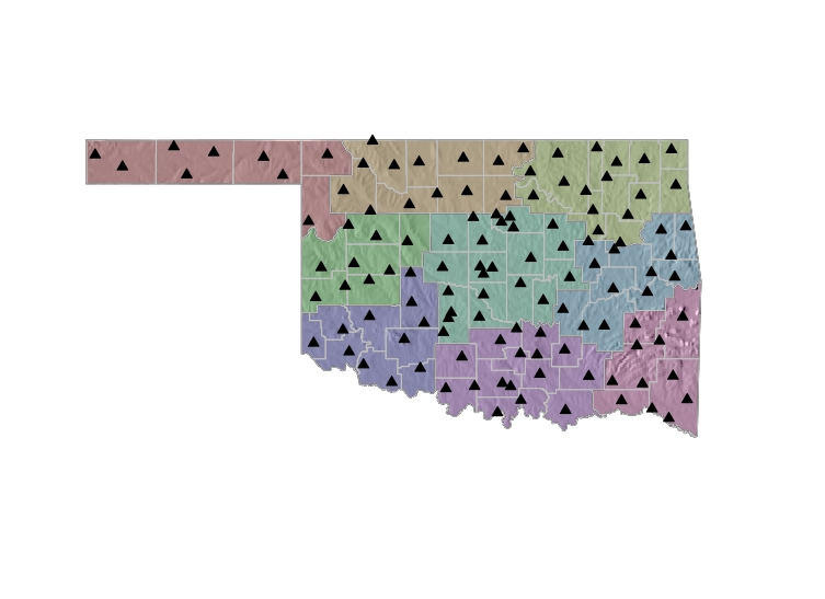
   Your advisor has tasked you with analyzing weather data from the Oklahoma Mesonet for an upcoming presentation. In particular, he is interested in the connection between weather and elevation. Since he knows you’ve been learning awesome data visualization and analysis tools in your scientific computing course he asks you to produce a map that shows the locations of all active Oklahoma Mesonet stations as well as the elevation, climate zones and county boundaries.

   Using install.packages(), install the raster, rgdal, and sp packages.

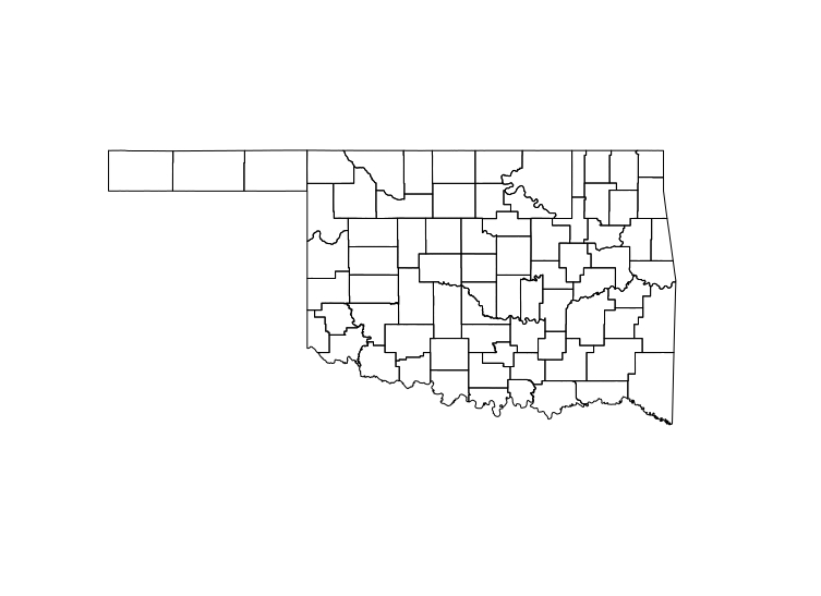
   1. You decide to start with a shapefile of the county boundaries. Download the Oklahoma county boundaries shapefile from here and the projection file from here. Unzip both files into your data directory. Use the readOGR function to read the county layer into R. Plot it using the plot function.

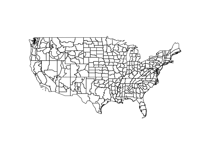
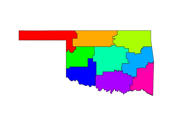
   2. Next you decide to read in a layer of the climate division boundaries. Download the zipfile of NOAA climate divisions from here and extract it in your data directory. Read in the GIS.OFFICIAL_CLIM_DIVISIONS layer and plot it using the plot function.

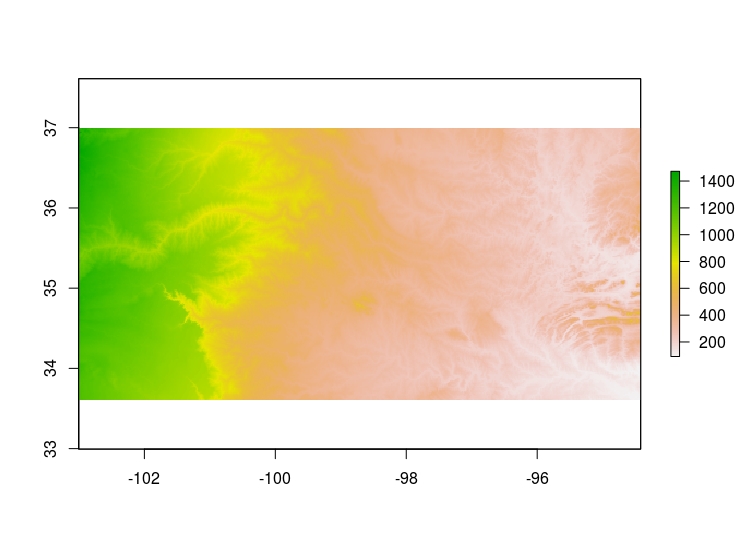
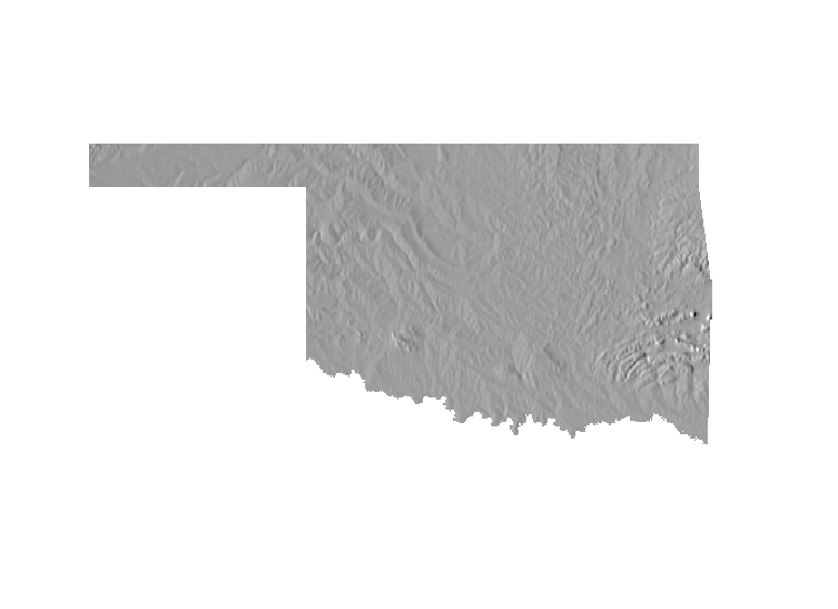
   3. Now that you’ve got the vector data layers imported, you decide to import a raster file of elevation for Oklahoma. Your friend has already clipped the National Elevation Dataset for Oklahoma agreggated it to a 1 arc-minute resolution, so she sends you a link to download it. Download it into your data folder and import it into R using the raster function. Plot the resulting data layer.

   [click here for output] [click here for output] [click here for output]

2. -- Converting Raw Data to Spatial Data --

   Your next task is to create a spatial data layer that contains the coordinates for Oklahoma Mesonet sites. You talk to your friend who has worked with Mesonet data before and she tells you about a handy R package called okmesonet for accessing Mesonet data. She suggests you use the updatestn function to pull in the station information you need.

   1. Install the okmesonet package and use the updatestn function to read in a data frame with the station location data. Use summary to check the data.

   2. On inspecting the data frame, you notice that some of the locations in the data frame have already been decommissioned. Because you are only interested in currently active stations, remove the rows for stations that have already been decommissioned. Check the data using summary.

   3. Now that you have the proper data, you need to convert your data.frame into a spatial data layer. You recall that in order to do this conversion you need to define a coordinate reference system (CRS) for the layer. Rather than create one from scratch you decide to extract the CRS from your county boundaries data layer, since that data set also uses latitude and longitude for coordinates. Use the crs function to extract the CRS from your county boundaries data layer and assign it to an R object.

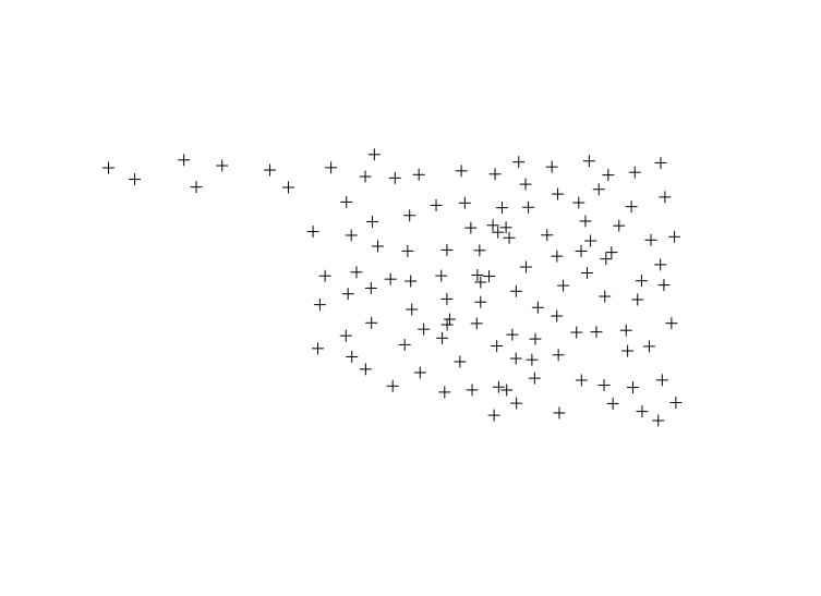
   4. Convert your data.frame to a SpatialPointsDataFrame using your CRS object and the SpatialPointsDataFrame function. Plot the resulting spatial data layer.

   [click here for output] [click here for output] [click here for output] [click here for output]

3. -- Manipulating and Transforming Spatial Data --

   Now that you have all the data in R, it’s time to prepare the data for creating your map. In order to create your map you need to have all of your layers clipped to the same extent and using the same projection.

   1. Use the extent function to check the geographic extent of the data layers for Oklahoma county boundaries, NOAA climate divisions, Oklahoma elevation, and Oklahoma Mesonet station locations.

   2. You note that all the layers seem pretty close except for the NOAA climate divisions and you realize that you forgot to subset that layer to include only climate divisions for Oklahoma. Use the subset function to exclude any polygons that are not in Oklahoma and assign the resulting SpatialPolygonsDataFrame to a new R object. Check the extent of the new data layer.

   3. Now that the extents are good, you need to check the projections. Use crs to check the projections of your data layers for Oklahoma county boundaries, Oklahoma climate divisions, Oklahoma elevation, and Oklahoma Mesonet station locations.

   4. You notice that the output from crs is different for your layers. To make sure that everything lines up properly you decide to transform each layer to match the CRS as specified for the Oklahoma county boundaries layer. Use spTransform to transform all your vector data layers to the CRS from the Oklahoma boundaries layer. Use crs to assign the proper CRS specification to your raster layer. Check all CRS specifications using crs.

   5. Plot all data layers starting with Oklahoma elevation. (Hint: use add=TRUE to overlay each data layer)

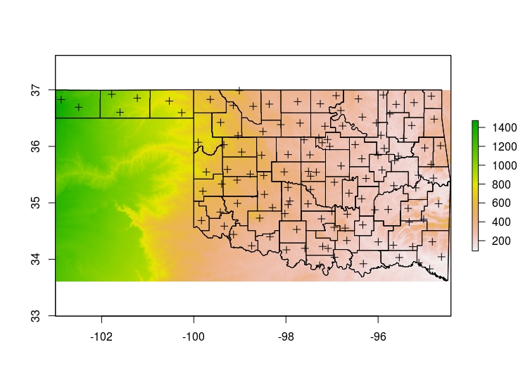
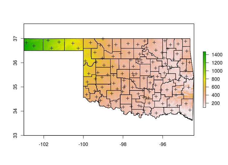
   6. In looking at your preliminary map, you realize that you need to remove the areas of the Oklahoma elevation data layer that are beyond the state boundary. Use the mask function to create a new data layer that contains only values that are within the state boundary. Plot all data layers starting with your new elevation data layer.

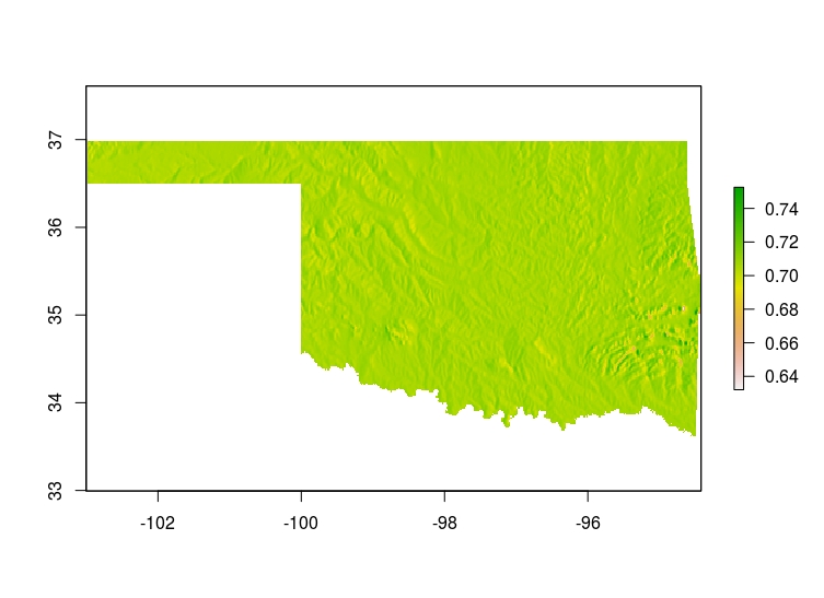
   7. You’re feeling pretty proud of your map so you show it off to your office-mate. He suggests that a hillshade plot for your elevation data might highlight the topography better. After some searching, you find that you can create a hillshade plot using the hillShade function. To do that, you’ll need to use the terrain function to calculate the slope and aspect and assign them to objects that you can provide as arguments to hillShade. Create a hillshade data layer using the slope and aspect calculated from the elevation data and plot the result. (Hint: use 45 for the angle and 270 for the direction arguments to hillShade)

   [click here for output] [click here for output] [click here for output] [click here for output] [click here for output] [click here for output] [click here for output]

4. -- Producing a Custom Map --

   Your data layers are ready to be combined into your final map.

   1. Plot the hillshade data layer.

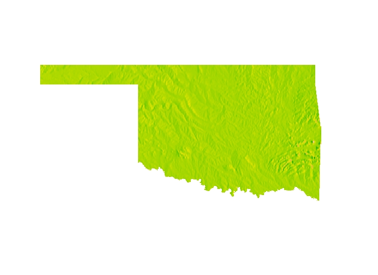
   2. The legend of the hillshade plot is not very informative and somewhat distracting so you decide it can be removed. You also decide that the axes and bounding box are unncessary. Plot the hillshade layer again removing the axes, bounding box, and legend. (Hint: use box=FALSE to get rid of the bounding box)

   3. Because you intend to overlay other layers on top of the hillshade layer, you decide it would be better to have the hillshade in grayscale instead of color. Use the gray function and the col argument to plot to plot the hillshade layer in grayscale. (Hint: using 0:100/100 for the level argument to gray should give you a nice contrast).

   4. Add the Oklahoma climate divisions to the map using the rainbow function and the col argument to plot. Be sure to specify the proper number of colors to correspond to the number of climate divisions when you call rainbow.

   5. You realize that in order to see the elevation you will need to increase the transparency of the colors for the climate divisions layer. Use the alpha argument to the rainbow function to make the colors more transparent and replot the elevation and climate division layers. (Hint: an alpha value of about 0.15 should be about right.)

   6. Now you are ready to add the Oklahoma county boundaries layer. Use plot to add this layer to the plot. The county boundaries are really more background context for the map, so use the border argument to set the color for the boundary lines to “gray”.

   7. You are now ready to add your Oklahoma Mesonet station locations to your map. Add the Oklahoma Mesonet station layer to your map. Use the pch argument to set the point character to a filled triangle.

   [click here for output] [click here for output] [click here for output] [click here for output] [click here for output] [click here for output] [click here for output]